Mechanically Modelling Eclipses
By Spencer Connor
Background
Eclipses are historically significant events for a combination of two things: their unique appearances and their apparent unpredictability. It’s no wonder that their striking but seemingly random appearances were attributed to theological causes for so long. But if you have a long enough period of observation, certain patterns start to emerge due to resonance of the various parameters needed for an eclipse. Famously, the Saros series can be used to predict eclipses with a moderate degree of accuracy as demonstrated by the Antikythera Mechanism. But it really isn’t comprehensive, and has a functional accuracy ceiling.
In this page, we’ll be exploring developing a mathematical model that could be implemented to produce an eclipse prediction machine. To get a basic understanding we must understand the basic geometry of an eclipse. Eclipses occur when the the sun, earth, and moon are located in a line (what astronomers called syzygy).
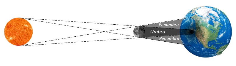
If the arrangement is Sun-Earth-Moon, this is a lunar eclipse and the moon will assume a reddish appearance as it passes into the earth’s shadow. You can see in the image on the right that the shadow of the earth is not a horizontal line, it is angled based on the relative sizes of the sun and earth (although far from to scale in the image). This splits the shadow into an umbra (where the entire sun is obscured) and a penumbra (where only some of the sun is obscured). With some simple geometry, we can find that the 2159 km moon has to pass through about a 5700 km umbral window for a total eclipse and about a 11,000 km penumbral window for a total eclipse. Way out 400,000 km away, that’s not a frequent occurrence.
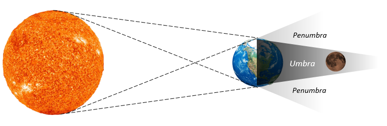
If the arrangement is Sun-Moon-Earth, this is a solar eclipse and the the sun will be obscured by the moon as a portion of the earth falls into the full or partial shadow of the moon. Again, the shadow splits into umbra and penumbra. The penumbra is about 2200 km, or roughly a third of the earth. The umbra varies from 98 km down to … -220 km. Wait, what does that mean? It turns out if the moon is far away (near apogee) the umbra will terminate before it hits the earth. Even if you stand at the center of the shadow, you’ll see the perimeter of the sun around the silhouette of the moon. This is called an annular solar eclipse.
So that doesn’t seem so complicated, why is it so hard to figure out when these happen?
While the sun doesn’t exactly move constantly through the sky either, the moon is overwhelming the issue. It is far from an ideal orbit, filled with all sort of precessions and perturbations that make it devilishly complicated to figure out where it will be at some point in the future especially years away. But it isn’t the only thing we need: to determine when an eclipse will occur and what it will look like, we need to be able to extrapolate three variables:
The position of the moon (relative to the fixed celestial sphere)
The position of the sun (relative to the fixed celestial sphere)
The apparent sizes of the moon and sun, which will determine the type of solar eclipse
For each of these variables, we’ll start with a simple model of the orbit, and compare it to the actual position/size in simulation (established from a modern planetarium software, Stellarium). We’ll look at why they aren’t matching, increase the complexity of our model to account for something we weren’t, and repeat until we are down to a reasonable accuracy. Then we will propagate our model way out to the next few eclipses, and see how close it is. Let’s start with the easier one…
1: Modeling the Position of the Sun
Model A: Circular Equatorial Orbit
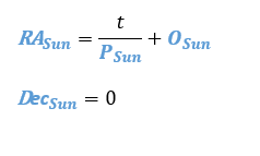
Starting simple is the best place to start. We know the sun moves through the stars with an average period of 365.25636 days (1 sidereal earth year). Let’s start by moving the sun through the celestial equator at a constant rate with this period. In astronomical terms, this means a constant change in right ascension of 360° per 365.25636 days or 0.9856 °/day. The declination remains constant at 0°.
Results
From the animation of the celestial sphere it’s pretty clear that the sun’s path is tilted over at an angle, and we are seeing an oscillating error in declination as a result. That bowling pin shape traced on the right has a very specific name, it’s called an analemma.
Making it Better
Let’s start with adding a tilt to the orbit so it’s not so obviously wrong, we can see the max declination error is 23.45° and hopefully that’s a familiar number if you’re interested in astronomy. It is the angle at which the earth is tilted, so our added tilt will be compensating for the earth being at an angle.
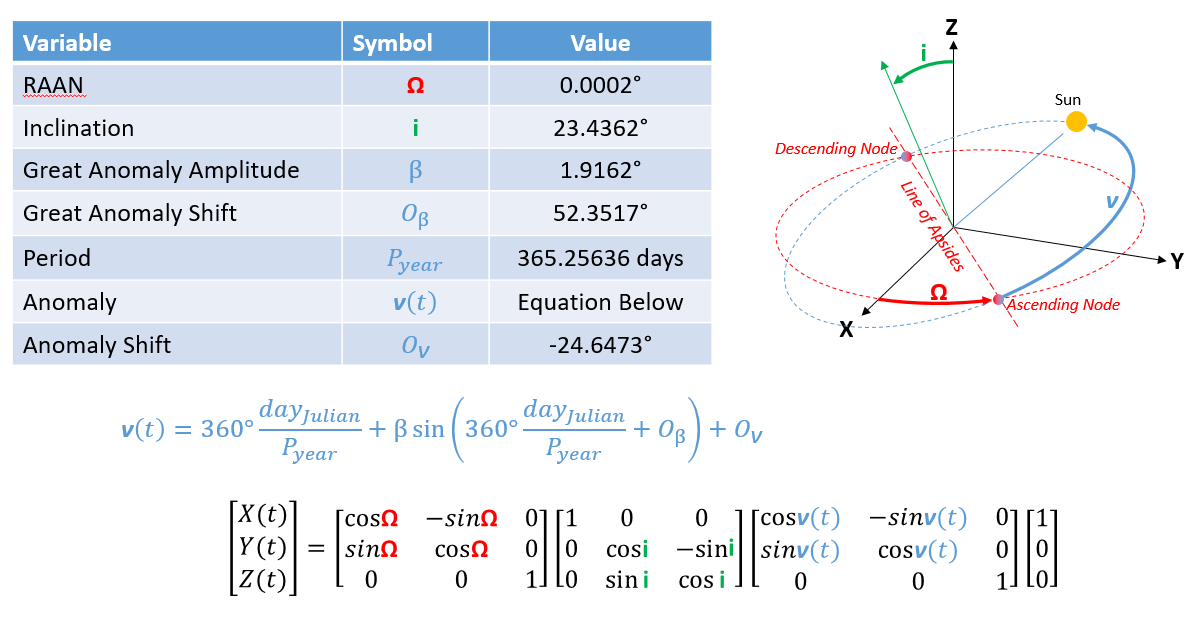
Model B: Circular Inclined Orbit
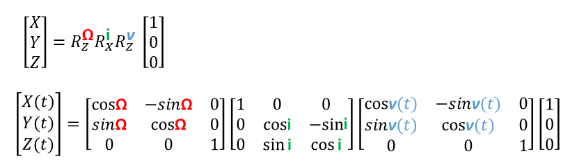
When an orbit is inclined, we need to know by how much and in what direction. If we pretend for a moment that the sun is orbiting the earth (cue 1400’s flashbacks…) we can use the classical Keplerian elements. The magnitude of the tilt is referred to as the inclination (i), as one might expect. The direction of the tilt is informed by a variable called the Right Ascension of the Ascending Node, or RAAN. Any tilted plane will intersect the equatorial (or XY) plane along exactly one line, referred to as the line of apsides. The orbit will cross this line at two points, one while passing from the bottom of the equatorial plane to the top and one while passing from the top to the bottom. These are called the Ascending Node and the Descending Node, and the Ascending Node is generally used as the orientation reference.
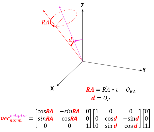
Now sequential transformation matrices are a little tricky, matrix multiplication is not commutative which means the order in which we build the transform matters. We are trying to get the position of object from its local frame to the inertial frame so we have to multiply its position by the LAST rotation matrix first.
Results
The tilt is matched very well with an inclination of 23.4° and a RAAN of 0°. The reason that the RAAN ends up at zero is that the zero reference for right ascension for everything is the vernal equinox, which is defined as the ascending node of the sun in this geocentric model. There is still a right ascension variation though, meaning a speeding up and slowing down of the sun throughout the year.
Making it Better
The Right Ascension variation is a result of eccentricity of Earth’s orbit, we’ll add that in with the next iteration of the model.
Model C: Eccentric Inclined Orbit
The eccentricity of the orbit produces more than just an oblong shape, it also produces uneven motion as a result of Kepler’s 2nd Law. Similar to the tilt of the orbit needing a parameter for magnitude and one for direction, the elongation of an orbit is defined by the eccentricity (0=circular, 1=on escape trajectory) and the argument of perigee. The variation in speed, and therefore position, that results is famous enough to have several names, among them The Great Anomaly and the Equation of the Center.
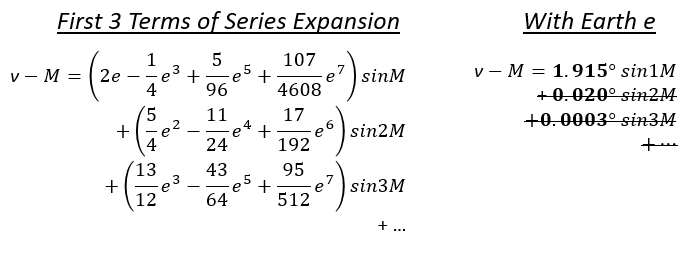
Now here we run into a bit of a problem for a physical machine modelling this…the timewise relationship of how much variation there is around the orbit is governed by Kepler’s Equation, which is a transcendental function. These are something of a mathematicians kryptonite, they don’t have algebraic solutions. Which means there is not going to be physical mechanism that perfectly emulates it, we are stuck having to make an approximation of our model that is an approximation of the truth! As discouraging as this is, you can get pretty close using something like the Antikythera Pin-Slot Assembly, and we are going to do even better here with a series expansion. On the right are the first three terms of the expansion in general form, and then with the earth eccentricity specifically. You can see that the magnitude of the terms quickly diminishes, so I’ll choose to include just the 1st term and accept the ~0.020° error as it is about 10x smaller than the sun diameter. This leaves us with a nice sinusoid that is easy to implement. The M in the equation is the Mean Anomaly with the same orbital period as the earth.
Results
That is looking much better, we are down to motion that is a small fraction of sun’s diameter. The remaining motion has some visible periodicity but it’s down to a level where the additional complexity of a mechanism to emulate it is not justified.
Wrapping Up Sun Position
Now we have a solar model that is of sufficient accuracy, extrapolation across 10 years shows the error stay bounded within 0.03 degrees and the star error pattern largely repeats on a yearly cycle. Below is the complete geometry of the model and the parameters determined via an optimization engine coded in MATLAB.
1: Modeling the Position of the Moon
Model A: Circular Equatorial Orbit
We’ll start the moon model the same way we did the sun model, with a simple circular equatorial orbit.
Results
Okay, well the good news is that the error is staying bounded across the 1 year simulation. But we’re seeing the same clearly apparent tilt to the orbit as we did with the sun.
Making it Better
The true orbit is significantly tilted and without accounting for it we are getting a huge oscillation in the declination (vertical) direction. Let’s correct that in our next model.
Results
There is a significant reduction in error, but not as much as the sun model. It looks like we’re going to have more terms to consider for the moon. Most of the residual motion is in the Right Ascension direction, as before.
Making it Better
We’ll need to compensate for the RA variation, but first we’re going to make a seemingly small correction up front while we’re digging into the inclination.
Isolating Lunar Orbit Vector With Linear Terms
If we assume a constant declination of the lunar orbit normal vector and a linearly changing right ascension we can compensate for the major motion. The best fit term for Right Ascension is a -0.053 °/day or one rotation in 18.6 years, matching the expected RAAN precession rate. The declination offset is 5.18°, close to the 5.15° expected. The residuals for both RA and declination appears to be approximately sinusoidal, let’s add in a sinusoidal term to both to address this next.
Model B: Circular Inclined Orbit
Next, we’ll add in the orbit plane tilt like the sun model, defined with an inclination and a RAAN. Note that the moon will have a non-zero number for the RAAN as it is not defining the First Point of Ares reference like the sun orbit.
Model C: Circular Precessing Inclined Orbit
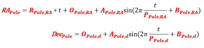
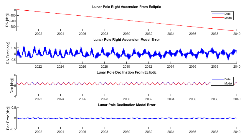
Now rather than going next to the equation of the center, we are going to tweak the inclination based on our knowledge of orbital mechanics. Recall that the inclination from the sun model was counteracting the earths axial tilt to get to an inertial plane. The axial tilt of the earth is essentially constant on the scale of decades. But the moon’s orbital plane is not aligned with the earth’s orbital plane, and our Model B of the moon is bundling both of those together. Which would normally just save us a step, EXCEPT that the RAAN of the moon is not constant. It precesses fairly quickly, once in about 18.6 years. So we’re going to break up the RAAN and inclination we found in Model B into RAAN/inclination to the inertial vector (as found in the Sun section) and the RAAN/inclination from the inertial vector to the moon orbit plane vector. The image on the right shows this effect, the moon’s orbit normal vector is not fixed like the sun but moving in a mostly circular path around a second vector. That second vector is the normal to the ecliptic, that we found when determining the inclination of the sun’s path. This simulation is across 20 years, so we get a bit more than the full 18.6 year precession. Moving forward, rather than working from the celestial coordinates we’ll go ahead and take out that static transform to the inertial ecliptic normal vector and just add it back in at the end.
Isolating Lunar Orbit Vector With Linear and Sinusoidal Terms
If we measure the period of both the RA and declination residuals we will find that they are almost exactly the same: 173.5 days. Now I’ll admit that the cause of this perturbation is not entirely clear to me, but this happens to be very, very close to the time between nodes of the earth (1/2 of the draconitic period of 346.62 days) so it does make some sense. At this point we have max RA and declination error of 0.66° and 0.052° respectively. The declination is the most important since it is the least coupled with the anomaly that we’ll evaluate next, that is known to have complex perturbations. So we’ll call this model good enough and move on to that.
Here we can see the sequel transforms from celestial to ecliptic, and then from ecliptic to lunar plane. While there is still a small amount of error in the declination direction, the nominal position is now almost entirely in a single plane so we can concentrate on the longitude (Right Ascension) terms specifically.
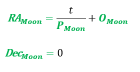
Moon Position in Lunar Plane with Linear Longitude Terms
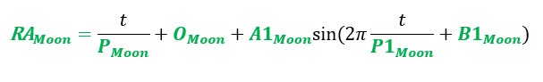
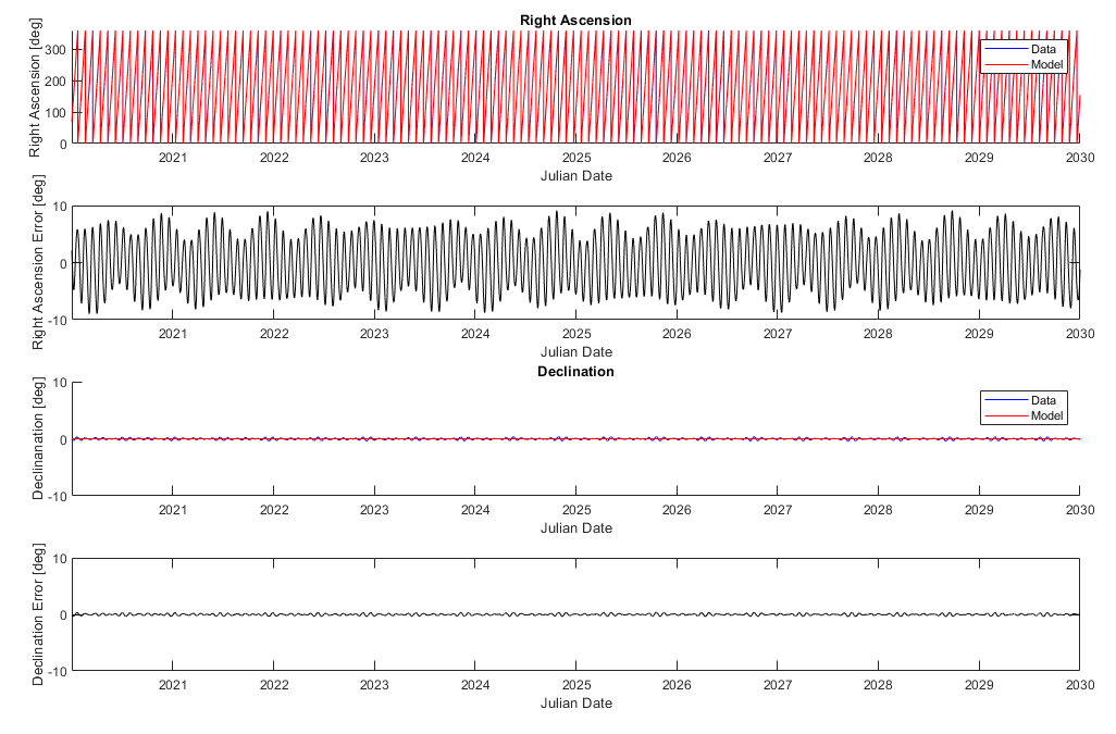
Starting with linear model of the longitude, using the equation shown below with a simple rate in the form of the sidereal period and an offset. From the Right Ascension Error plot (2nd down) it’s clear that the linear model leaving ~10° of error will need some refinement with oscillating terms, but the declination is down to a pretty reasonable level from our effort getting the plane established. The Right Ascension error has clearly visible multiple sinusoidal terms layered, so we’ll next try to isolate some frequencies to start adding in signals
Adding a Sinusoidal Term to Longitude
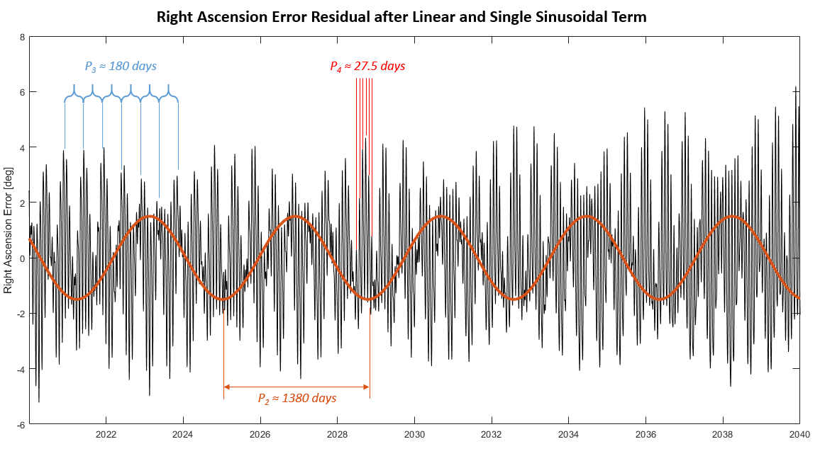
The primary frequency to be taken out corresponds to a 27.5662 day period, so we’ll run a curve fitting function with that criteria to find our amplitude (A1) and offset (O1) and then subtract that out of our residual. There are still clearly multiple oscillating signals present in the residual, just by eye I could see three at about 1380, 180, and 27.5 days.
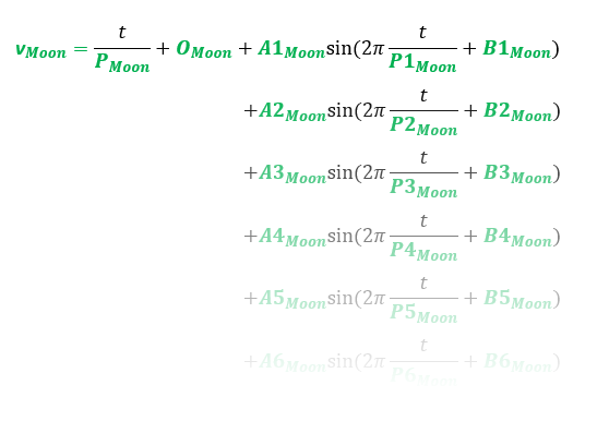
Adding More Sinusoidal Terms
Starting with residual from the previous section and the estimates for the period for the next three sinusoidal frequencies, we’ll run the data through an optimization against an equation of the form shown on the right to solve for the true periods as well as the phase (O) and amplitude (A) of each of the terms. Note that this is consider the linear and first oscillating term frozen and will not yield us a globally optimized solution. The reason for that MATLAB’s fminsearch function isn’t great at avoiding local minima and our goal function is minimizing the max error over then entire timespace. As the inputs are varied, different times become the places of max error, so the error gradient becomes highly discontinuous and the optimization needs to be close to the solution to confidently find the error minimum. Incrementally adding the terms like this allows us to manually guide it towards the solution, and at the end we can run it simultaneously to make sure we are truly in a minimum.
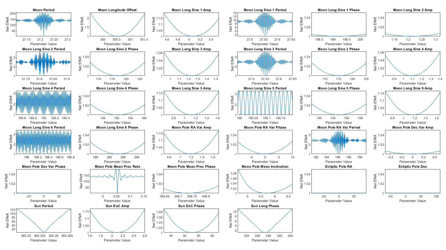
Global Optimization and Changing the Goal
Next, we integrate our sun and moon motion models together and run global optimization. This means we are simultaneously tweaking every variable we have come up with thus far and driving our new goal, the difference between the sun-to-moon angle of the true data vs. our model, down to a minimum. We have to consider the entire time range here for every step, and with 34 variables in play this is a calculation to run overnight. Overall, the optimization called the error function around 7 million times with different combinations of parameter values, each time building the model across the 50 year span and and comparing it at every hour to the true data. The results are shown on the right. Every variable is centered on a minimum that will cause an increase in error if moved in either direction. Note that some variables actually become inconsequential and become candidates to eliminate from the model with no negative effect. For example, the Ecliptic Pole location ends up not mattering because it is shared by the moon and sun position models and any error will cancel out.

1: Combining Sun and Moon Position Models
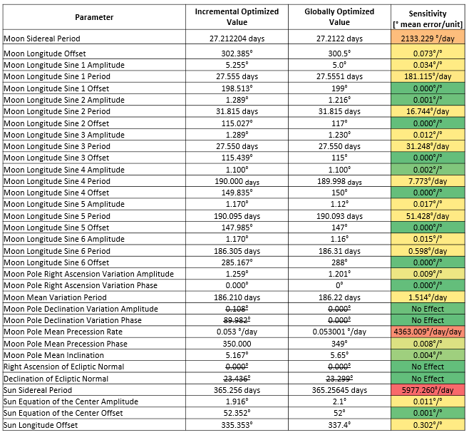
Sensitivities
For building a mechanical model, it is important to understand the sensitives of each variable (how much a variation in it will produce variation in the end result). High sensitivities need tight tolerances and alignments, low sensitivities less so. Not that these sensitivities are unilateral, assuming all other parameters are fixed. In reality there is some coupling between them, which could be addressed through more complex methods like Monte Carlo analyses if desired. I’ve highlighted the sensitivities by magnitude and it’s plainly visible that the rate terms are the most critical to get accurate, which makes sense as error in those will compound unbounded over time. Also note that the Moon Pole declination magnitude was optimized to zero, so the phase doesn’t matter. We’ll eliminate this term in the final model, as the effect it was capturing ended up being better address by other terms during our global optimization.
Final Parameters

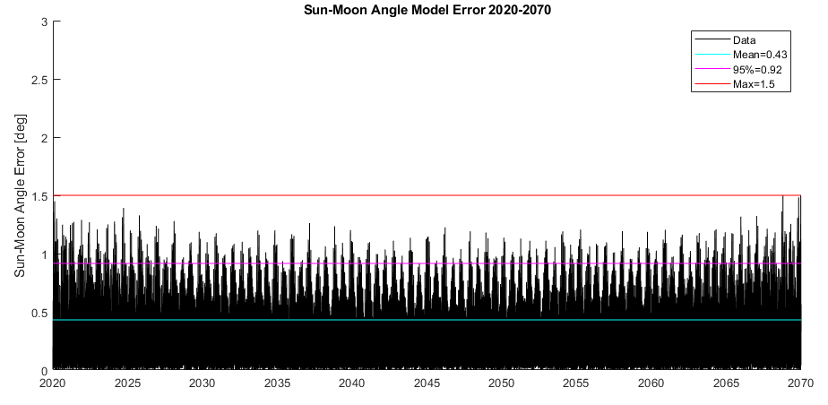
Assessing Accuracy with Sun-Moon Angle Error
Now’s the nerve-racking point where we seen if all our estimates of “close enough” were indeed good enough. We’ll start with a general examination of the accuracy of the moon-to-sun angle. We get a mean error of 0.43°, a 95% deviation of 0.92°, and a maximum error of 1.50°. For comparison, the moon and sun diameters are about half a degree so if we were getting more than a degree of sustained error there would be little chance of predicting eclipses with this model. As it stands there is error of course, but an acceptable amount.
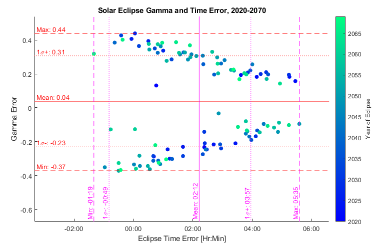
Assessing Accuracy at Known Solar Eclipses
But now let’s run the REAL test, how well DOES it predict eclipses? We’ll run through every solar eclipse in the 21st century and compare the timing and gamma of the eclipse.
Gamma describes how “on center” the eclipse is:
0 is right through the center of the earth
1 is just skimming one of the poles
1- 1.55 will yield a partial eclipse as the penumbra still hits the earth
>1.55 means even the penumbra misses and there is no eclipse.
From the results below we see the model is doing very well, there will always be some cases where the model and true data are straddling the threshold for either total or partial eclipse but there are not instances where the model entirely misses a total eclipse (which would require a gamma error of 1). If we look at the errors in aggregate on the right the error is has no visible correlation over time, so the model does not appear to be degrading which is good. It does tend to predict the eclipse as occurring a couple hours late (which can be handled with a simple universal time offset at the input). The gamma error has a strong mirror pattern, with two error zones slanted to correspond to the eclipses at the ascending and descending nodes. Overall, the accuracy of this model is better than anticipated. However, we must also keep in mind that there will be additional degradation when physically implemented into a mechanical model. Until then, happy eclipsing!